


Memory reduction for average-link Hierarchical Clustering
In this article, we will consider the usage of the agglomerative approach to hierarchical clustering – a method of cluster analysis that seeks to build a hierarchy of clusters.
Hierarchical clustering (also called hierarchical cluster analysis or HCA) is a method of cluster analysis that seeks to build a hierarchy of clusters. Approaches to hierarchical clustering are typically reduced to two types:
- Agglomerative: this is a "bottom-up" approach, where each observation starts in its own cluster and the pairs of clusters are merged as one moves up the hierarchy
- Divisive: this is a "top-down" approach, where all observations start in one cluster, and splits are performed recursively as one moves down the hierarchy
In this article, we will consider the usage of the Agglomerative type.
Generally, the merges are produced in a “greedy” manner. And the results of hierarchical clustering are usually presented in a dendrogram.
The complexity of agglomerative clustering is estimated as O(N3), which explains the low speed of working with large data sets. However, there can be a more efficient method of realization for some special cases.
Suppose that there is a set of N items to be clustered. Then, there will be an NxN distance matrix and the basic process of hierarchical clustering will consist of the next steps:
Each element is assigned to a separate cluster, i.e. the number of clusters will be initially equal to the number of elements. It is assumed that the distance between the clusters is the distance between the elements they contain.
- The clusters closest to each other are paired. They turn into one new cluster.
- The distance between the new and old clusters computes according to the described method.
- The second and third steps are repeated until there is a cluster containing all the elements.
- The third step can be implemented in several ways: single-link, complete-link and average-link clustering.
We will consider an average-link clustering algorithm.
In average-link clustering, the distance between the clusters is determined by the average distance between their elements.
There is an existing average-link hierarchical clustering algorithm with the complexity of O(N2*log N), which requires storing O(N2 * (2 * sizeof(dataType) + sizeof(indexType)) elements. We used the same approach to improve the algorithm’s complexity, but this implementation requires storing only O(N2 * (sizeof(dataType) + 2 * sizeof(indexType))) elements, where size of(dataType) > sizeof(indexType).
Example #1
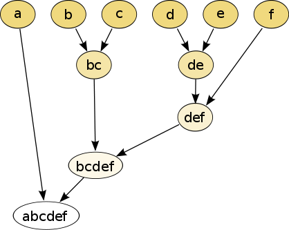
Abstract raw data before building a dendrogram.
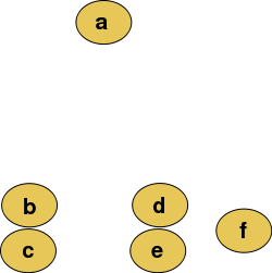
The hierarchical clustering dendrogram will look like this after the algorithm running:
Algorithm improvements
The initial algorithm has some issues with large amounts of data. So we applied the next improvements to minimize the processing time and memory consumption.
-
All the information is stored only for unused elements (including those that were produced by combining). As the matrix of distances is symmetric, all calculations and operations are produced by its lower triangular shape.
           public float getCopheneticCorrelation(float[][] matrix) {
             matrix = Utils.toTriangularMatrix(matrix);
             Dendrogram dendrogram = getDendrogram(matrix);
             …
          }
activeRows = new TIntNSet(totalRowsCount); for (int row = 0; row < rowsCount; ++row) { activeRows.addLast(row); }We deactivate two rows, and activate a new one, which is the result of merging the ones we’ve deactivated.
          …
        deactivateRow(minRow);
        deactivateRow(minRowColumn);
        …
… activateRow(addedRow); … protected void deactivateRow(final int row) { activeRows.remove(row); tree.set(row, 0); } protected void activateRow(final int row) { activeRows.addLast(row); tree.set(row, 1); } -
Because the used matrix is a lower triangular shape and sorted in each row elements, it becomes impossible to update the elements’ distance to the new cluster in O(1) without a memory increase. Therefore, we add a new option (that saves the layout of the elements after sorting) to avoid this.
this.rowColumns = new TShortIntArray[totalRowsCount]; //columns before sorting this.rowColumnIndexes = new TShortIntArray[totalRowsCount]; //column positions after sorting for (int row = 0; row < rowsCount; ++row) { Utils.DoubleValueIndexPair[] pairs = new Utils.DoubleValueIndexPair[row]; for (int column = 0; column < row; ++column) { pairs[column] = new Utils.DoubleValueIndexPair(matrix[row][column], column); } Arrays.sort(pairs); rowColumns[row] = new TShortIntArray(row, row); rowColumnIndexes[row] = new TShortIntArray(row, row); for (int index = 0; index < row; ++index) { int column = pairs[index].index; rowColumns[row].setValue(index, column); rowColumnIndexes[row].setValue(column, index); } } -
We can use the information about the deactivated rows for getting the correct index of the needed column position in the third parameter. The initial complexity of this operation is O(N). However, we can reduce the complexity to O(log N) by using the segment tree structure.
-
However, the segment tree structure increases memory consumption. Each added cluster requires a separate version of a tree, which in its turn requires O(N2) memory (thus up to O(N3) in general). Therefore, we added persistency to the segment tree structure for optimization. This approach will minimize memory consumption up to O(log N). It will be very significant when working with a large amount of data.
this.tree = new TPersistentSumSegmentTree(states, maxChangesCount);We get the distance from both elements and then get an average distance to merge them.
          float minRowDistance = getDistance(minRow, currentRow);
          float minColumnDistance = getDistance(minRowColumn, currentRow);

          float addedRowDistance = getMergedDistance(minRow, minRowDistance, minRowColumn, minColumnDistance, addedRow);
          protected int getColumnIndex(int row, int column) {
             if (row < rowsCount) {
                return column;
             }

             int changeRootIndex = (row - rowsCount + 1) * 3;
             int columnIndex = tree.getSum(changeRootIndex, 0, column) - 1;

             return columnIndex;
          }
protected float getMergedDistance(int left, float leftDistance, int right, float rightDistance, int root) { float rootDistance = leftDistance * sizes[left] + rightDistance * sizes[right]; rootDistance /= sizes[root]; return rootDistance; }
Example #2
The next pages trace a hierarchical clustering of distances in miles between U.S. cities.
Input distance matrix:
|
|
BOS |
NY |
DC |
MIA |
CHI |
SEA |
SF |
LA |
DEN |
|
BOS |
0 |
|
|
|
|
|
|
|
|
|
NY |
206 |
0 |
|
|
|
|
|
|
|
|
DC |
429 |
233 |
0 |
|
|
|
|
|
|
|
MIA |
1504 |
1308 |
1075 |
0 |
|
|
|
|
|
|
CHI |
963 |
802 |
671 |
1329 |
0 |
|
|
|
|
|
SEA |
2976 |
2815 |
2684 |
3273 |
2013 |
0 |
|
|
|
|
SF |
3095 |
2934 |
2799 |
3053 |
2142 |
808 |
0 |
|
|
|
LA |
2979 |
2786 |
2631 |
2687 |
2054 |
1131 |
379 |
0 |
|
|
DEN |
1949 |
1771 |
1616 |
2037 |
996 |
1307 |
1235 |
1059 |
0 |
The nearest pair of cities is BOS and NY at a distance of 206. These are merged into a single cluster called "BOS/NY".
Then, we compute the distance from this new compound object to all other objects. The distance from "BOS/NY" to DC is 331 and it corresponds to the average distance from NY and BOS to DC. Similarly, the distance from "BOS/NY" to DEN will be 1,860.
After merging BOS with NY:
|
|
BOS/NY |
DC |
MIA |
CHI |
SEA |
SF |
LA |
DEN |
|
BOS/NY |
0 |
|
|
|
|
|
|
|
|
DC |
331 |
0 |
|
|
|
|
|
|
|
MIA |
1406 |
1075 |
0 |
|
|
|
|
|
|
CHI |
882.5 |
671 |
1329 |
0 |
|
|
|
|
|
SEA |
2895.5 |
2684 |
3273 |
2013 |
0 |
|
|
|
|
SF |
3014.5 |
2799 |
3053 |
2142 |
808 |
0 |
|
|
|
LA |
2882.5 |
2631 |
2687 |
2054 |
1131 |
379 |
0 |
|
|
DEN |
1860 |
1616 |
2037 |
996 |
1307 |
1235 |
1059 |
0 |
The nearest pair of objects is BOS/NY and DC at a distance of 331. These are merged into a single cluster called "BOS/NY/DC". Then, we compute the distance from this new cluster to all other clusters to get a new distance matrix:
After merging DC with BOS-NY:
|
|
BOS/NY/DC |
MIA |
CHI |
SEA |
SF |
LA |
DEN |
|
BOS/NY/DC |
0 |
|
|
|
|
|
|
|
MIA |
1240.5 |
0 |
|
|
|
|
|
|
CHI |
776.75 |
1329 |
0 |
|
|
|
|
|
SEA |
2789.75 |
3273 |
2013 |
0 |
|
|
|
|
SF |
2906.75 |
3053 |
2142 |
808 |
0 |
|
|
|
LA |
2756.75 |
2687 |
2054 |
1131 |
379 |
0 |
|
|
DEN |
1738 |
2037 |
996 |
1307 |
1235 |
1059 |
0 |
Now, the nearest pair of objects is SF and LA at a distance of 379. These are merged into a single cluster called "SF/LA". Then we compute the distance from this new cluster to all other objects to get a new distance matrix:
After merging SF with LA:
|
|
BOS/NY/DC |
MIA |
CHI |
SEA |
SF/LA |
DEN |
|
BOS/NY/DC |
0 |
|
|
|
|
|
|
MIA |
1240.5 |
0 |
|
|
|
|
|
CHI |
776.75 |
1329 |
0 |
|
|
|
|
SEA |
2789.75 |
3273 |
2013 |
0 |
|
|
|
SF/LA |
2831.75 |
2870 |
2098 |
969.5 |
0 |
|
|
DEN |
1738 |
2037 |
996 |
1307 |
1147 |
0 |
Now, the nearest pair of objects is CHI and BOS/NY/DC at a distance of 776.75. These are merged into a single cluster called "BOS/NY/DC/CHI". Then, we compute the distance from this new cluster to all other clusters to get a new distance matrix:
After merging CHI with BOS/NY/DC:
|
|
BOS/NY/DC/CHI |
MIA |
SEA |
SF/LA |
DEN |
|
BOS/NY/DC/CHI |
0 |
|
|
|
|
|
MIA |
1284.75 |
0 |
|
|
|
|
SEA |
2401.375 |
3273 |
0 |
|
|
|
SF/LA |
2464.875 |
2687 |
808 |
0 |
|
|
DEN |
1367 |
2037 |
1307 |
1147 |
0 |
Now the nearest pair of objects is SEA and SF/LA at distance 808. These are merged into a single cluster called "SF/LA/SEA". Then, we compute the distance from this new cluster to all other clusters to get a new distance matrix:
After merging SEA with SF/LA:
|
|
BOS/NY/DC/CHI |
MIA |
SF/LA/SEA |
DEN |
|
BOS/NY/DC/CHI |
0 |
|
|
|
|
MIA |
1284.75 |
0 |
|
|
|
SF/LA/SEA |
2433.125 |
2980 |
0 |
|
|
DEN |
1367 |
2037 |
1227 |
0 |
Now, the nearest pair of objects is DEN and SF/LA/SEA at a distance of 1,227. These are merged into a single cluster called "SF/LA/SEA/DEN". Then, we compute the distance from this new cluster to all other clusters to get a new distance matrix:
After merging DEN with SF/LA/SEA:
|
|
BOS/NY/DC/CHI |
MIA |
SF/LA/SEA/DEN |
|
BOS/NY/DC/CHI |
0 |
|
|
|
MIA |
1284.75 |
0 |
|
|
SF/LA/SEA/DEN |
1900.063 |
2508.5 |
0 |
Now the nearest pair of objects is BOS/NY/DC/CHI and MIA at a distance of 1,284.75. These are merged into a single cluster called "BOS/NY/DC/CHI/MIA". Then, we compute the distance from this new compound object to all other objects to get a new distance matrix:
After merging BOS/NY/DC/CHI with MIA:
|
|
BOS/NY/DC/CHI/MIA |
SF/LA/SEA/DEN |
|
BOS/NY/DC/CHI/MIA |
0 |
|
|
SF/LA/SEA/DEN |
1896.625 |
0 |
Finally, we merge the last two clusters at level 1896.625.
In this article, we reviewed the following aspects:
- The original hierarchical clustering algorithm
- Algorithm modifications, decreasing the algorithm’s complexity from O(N3) up to O(N2 log N)
- Modifications that allow for decreasing the amount of used memory from O(N3) up to O(N2 log N) without increasing the algorithm’s complexity up to the original O(N3)
- Example of a general algorithm
References
- D'andrade,R. 1978, "U-Statistic Hierarchical Clustering" Psychometrika, 4:58-67
- Johnson,S.C. 1967, "Hierarchical Clustering Schemes" Psychometrika, 2:241-254
- Kaufman, L.; Rousseeuw, P.J. (1990). Finding Groups in Data: An Introduction to Cluster Analysis (1 ed.). New York: John Wiley. ISBN 0-471-87876-6
- http://nlp.stanford.edu/IR-book/html/htmledition/time-complexity-of-hac-1.html
If you need development assistance in a similar project or you have questions about the algorithm implementation, please write to us at hello@wave-access.com and our experts will help you.
Let us tell you more about our projects!
Сontact us:
hello@wave-access.com


